Smooth ACT policies on the SO101 arm
This blog post introduces ACTSmooth, a custom ACT policy for smoother trajectories. ACTSmooth extends ACT with prefix conditioning and async inference, eliminating inter-chunk discontinuities and inference latency stalls. I’m focusing on ACT on the SO101 arm because it has become the hello world of robot learning, thanks to LeRobot, but the default implementation suffers from jerky motions. Async inference and real-time chunking (RTC) address smoothness for policies with diffusion or flow matching action heads. I wanted to see if I could apply these ideas to ACT, where actions are produced in a single forward pass.
In teleoperation, a human moves a leader arm and a follower arm tracks its position. There’s noise due to latency (~100ms in my setup), overshoot, undershoot. ACT takes the follower’s joint positions and camera images as input and outputs a chunk of leader positions: the actions the follower must track. It is trained to minimize the distance to the trajectory commanded by the human during data collection, which is typically smooth. The problem is that no information about previously commanded actions reaches the policy, only the noisy follower position does. This makes it hard to output leader positions that are smooth continuations of the previously commanded leader positions, and jerkiness in the commanded trajectory becomes jerkiness in the robot’s motion. ACTSmooth passes the last few actions of the commanded trajectory as additional input, giving the policy what it needs to surface the smoothness already present in the human demonstrations. ACT has no denoising process to enforce continuity with the last few commanded actions; ACTSmooth just relies on the human bias toward smooth motion.
Smoothness matters. For position-controlled arms like the SO101, the PID controller responds to error: the gap between where the joint is and where you want it to be. A sudden jump creates a large instantaneous error; the servo will attempt to close the gap fast. This causes peak torque and heat in the motor, along with vibrations as the controller overshoots and settles. At the task level this translates to missed grasps, lost contact, collisions. Moreover, since policies train on smooth human demonstrations, jerkiness during inference shifts the observation distribution away from what the model has seen during training.
Contents
Background
Action Chunking with Transformers (ACT) takes camera images and robot proprioception as input and outputs a chunk of C actions (C = 30 and C = 10 in the experiments below). For data collected through teleoperation, the actions are the absolute joint positions of the leader arm, which the follower then tracks. The policy is trained to minimize the L1 distance between the predicted chunk and the ground-truth leader positions. Data is collected at a fixed FPS (30FPS and 10FPS in the experiments below); each timestep has one observation and one action, and during inference actions are commanded at the same rate.
Two distinct problems arise when running the policy in the real world:
- Inference latency. During training ACT learns to predict action chunks where the first action’s timestep corresponds to the input observation’s timestep. But when running the policy there is an unavoidable delay between capturing the observation and executing the first predicted action: inference alone generally takes tens or hundreds of milliseconds. In our setup, a single ACT forward pass takes around 40ms, which means that, for a policy running at 30fps, at least two timesteps elapse before the first action can be executed.
- Inter-chunk discontinuities. Each action chunk is predicted independently, from the current state of the robot and of the environment. A smooth handoff would require the next chunk to begin in proximity of where the previous one ends. But this often doesn’t happen since consecutive chunks have no knowledge of each other. Instead, the robot jumps discontinuously at chunk boundaries.
These two problems compound. Longer delays mean staler observations, which means that the head of each next chunk is predicted from a state the robot has already drifted away from, producing a bigger jump. The methods below address both issues, with increasing sophistication, changing the model, the inference script (which runs model inference and commands actions to the real robot), or both.
Synchronous inference
The default. The robot pauses while inference runs, then executes the action chunk. This creates visible stalls.
loop:
  obs = get_observation()
  chunk = policy(obs) # robot stalls during inference
  for action in chunk:
    execute(action)
    sleep(1/fps)
Synchronous inference with latency matching
The approach in the UMI paper. It explicitly measures inference latency and discards the first few actions in the next chunk that correspond to timesteps already elapsed during inference. This fixes the temporal misalignment and avoids executing stale actions, but it still implies a pause during inference. The cost is often larger discontinuities between chunks, since actions later in the chunk tend to move the robot further away from its position when the observation was captured.
UMI also separately compensates for observation and execution latencies, which matter when data collection and inference happen on different hardware. We assume a teleoperation setup, where we don’t have to deal with this complexity.
loop:
  obs = get_observation()
  chunk = policy(obs) # robot stalls during inference
  skip = ceil(duration_inference / duration_frame)
  for action in chunk[skip:]:
    execute(action)
    sleep(1/fps)
Synchronous inference with temporal ensembling
The approach in the original ACT paper. The policy is evaluated every timestep rather than once per chunk. Actions from different chunks that cover a specific timestep are averaged, weighted exponentially by recency. This smooths chunk boundaries without any model changes.
Two problems make temporal ensembling unattractive in practice. First, if consecutive predictions commit to different modes (e.g. getting around an obstacle either from the left or from the right) the averaging produces a trajectory that is none of the valid options (potentially driving into the obstacle). Second, it adds C - 1 inference calls and therefore wastes compute compared to other inference methods.
Asynchronous inference with latency matching
Async inference decouples action execution from policy inference by running them on two separate threads. The actor thread runs at the robot’s control rate (e.g. 30fps) and continuously executes actions from the active chunk. The inference thread runs policy inference in the background, when it finishes the new chunk is queued as pending. The actor thread switches to the pending chunk when it arrives, before the active chunk is exhausted, discarding stale actions the same way as in synchronous inference with latency matching. This eliminates stalls and keeps the robot moving continuously. However, inter-chunk discontinuities remain: consecutive chunks still don’t know about each other.
The following implementation is a simplification of the original async inference logic.
# actor thread
loop:
  obs = get_observation()
  if chunk_pending.action_at(timestep) exists:
    chunk_active = chunk_pending
  action = chunk_active.action_at(timestep)
  execute(action)
  if chunk_active.actions_remaining <= threshold:
    request_inference(obs)
  timestep += 1

# inference thread
loop:
  wait_for_request()
  chunk_pending = policy(obs)
Actions in a chunk are indexed by timestep. During training, the first action in a chunk corresponds to the observation’s timestep, so each chunk stores chunk.timestep_obs and chunk.action_at(timestep) returns the timestep - chunk.timestep_obs-th action. chunk.action_at(timestep) returns nothing if no chunk is pending or if the timestep falls outside the chunk. This makes skipping stale actions automatic: when the actor switches to the pending chunk, it calls action_at with the current timestep and lands at the right position, skipping any actions corresponding to timesteps elapsed during inference.
The threshold controls how early the inference is triggered: you want to start inference with enough actions remaining in the active chunk to execute while it runs. The right value depends on the measured inference latency of your system.
We limit our analysis to inference and robot control happening on the same physical machine, but async inference can be extended to server-client architectures where inference happens on a remote GPU server.
Asynchronous inference with inference-time RTC
Inference-time RTC poses asynchronous inference as an inpainting problem. The first few actions of the next chunk, those already committed to execution while inference runs, are frozen to match the previous chunk. The remaining actions are inpainted by the flow matching denoising process, guided to be consistent with the frozen prefix. The method works with any diffusion or flow-matching policy out of the box, requiring no retraining. The downside is added inference latency from the guidance computation at each denoising step. The math is also fairly complicated.
Because the inpainting relies on guiding the denoising process, it has no direct analog for ACT, which produces actions in a single forward pass.
Asynchronous inference with training-time conditioning
Train (or fine-tune) a policy conditioned on a prefix of actions from the previous chunk. The trajectories collected from human demonstration, which the policy is trained on, are smooth. By passing information from the previous chunk, the policy is biased towards this smoothness, learning to avoid discontinuities at chunk boundaries. During inference, we pass the last few actions from the previous chunk as prefix, those already committed to execution while inference runs.
Training-time RTC frames prefix conditioning as simulated inference delay. During training, sample a random delay d, treat the first d actions of the chunk as the prefix, and supervise only on the postfix. In the denoising process, prefix positions are treated as fixed tokens while postfix positions are noisy tokens. The model only predicts and is supervised on the postfix. On top of the smoothness coming from the human demonstration, this setup for the denoising process further biases the policy towards outputting continuous continuations from the prefix. The method requires no architecture changes and can be applied as a fine-tune on an existing checkpoint. Unlike inference-time RTC which adapts at runtime, it has no inference-time overhead but the delay distribution must be fixed at training time based on expected inference latency.
VLASH rolls the robot state forward using the already-committed actions and feeds this future state as proprioception to the model. If you know which actions the robot will execute and the current joint positions, you can compute where the arm will be when the next chunk takes over. A random delay is sampled during training so that the model learns to handle the full range of expected inference latencies. VLASH employs block-sparse attention to efficiently train on multiple delay values in a single forward pass. One thing to note is that only the proprioception is rolled forward, not the camera images. A limitation compared to training-time RTC is that the model does not receive information about the trajectory shape and velocity of the previous chunk, just about its endpoint position.
Another recent work exploring this direction is REMAC (which also extends to ACT).
ACTSmooth takes the future prefix conditioning from training-time RTC and the efficient multi-delay training from VLASH, and brings them to ACT.
ACTSmooth
At the model level, ACTSmooth extends ACT with prefix conditioning and relative action representation, both of which pass information from the previous chunk to the policy. ACT has no flow-matching action head; instead, it outputs actions in a single forward pass. We cannot rely on the denoising process to enforce smooth continuations of the prefix, but we can still allow the policy to surface the smoothness of human demonstrations by conditioning on information about the previous chunk.
We distinguish between future and past prefix conditioning. During training, future prefix actions correspond to timesteps at or after the input observation timestep; past prefix actions correspond to earlier timesteps. During inference, as future prefix we pass the actions of the previous chunk that are committed to execution while inference runs but have not been commanded yet; as past prefix we pass actions of the previous chunks that have been commanded already.
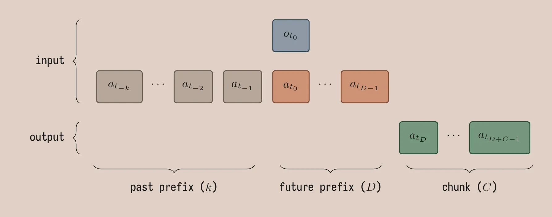
Future prefix conditioning. This is directly analogous to training-time RTC: condition the policy on d actions from the previous chunk. The model predicts a chunk of length C starting after the prefix. During training, d is sampled from \{1, \ldots, D\}, so the model learns to handle any delay up to D timesteps. The minimum d \geq 1 encodes the idea that there is always at least one frame of latency because of a training/inference mismatch: the first action a_{t_0}, corresponding to the observation o_{t_0}, cannot be executed immediately on the robot because there is always some greater-than-zero inference latency.
Past prefix conditioning. The past prefix consists of k actions from before the observation timestep. It allows the model to read how fast and in which direction the arm is moving to produce smoother continuations. The past prefix also decouples the total prefix length from the system’s inference latency: k is a free design choice to provide more history information to the policy, independently of d which is set based on measured inference latency.
Relative action representation. We replace the absolute joint positions with joint positions relative to the last action in the prefix a_{t_0}. The relative representation biases actions at the start of the chunk toward zero. In smooth human demonstrations, early actions in a chunk are typically close to the anchor action. This is easier to learn for the model when working with relative joint positions, where it learns to output small offsets, compared to absolute joint positions, where it would have to learn to compute subtractions internally to make sure the actions are close to the input prefix. Note that the anchor is the commanded action a_{t_0}, not the robot’s observed state o_{t_0}. We also tried anchoring on o_{t_0} and it worked qualitatively worse, but we don’t have an ablation.
Implementation details
Both past and future prefix tokens are added as inputs to the encoder. The token sequence is [image features, latent z, robot state, past prefix, future prefix]. The decoder is unchanged from standard ACT: C tokens cross-attend to the encoder output, each mapping to an action; the CVAE structure is also preserved. The L1 loss is computed on the postfix for all D delay values simultaneously: for delay d, the target actions are a_{t_0+d}, \ldots, a_{t_0+d+C-1}, and the loss is averaged across all D delays, all C timesteps, and the batch.
During training, rather than sampling one delay d per sample in the batch, we evaluate all delay values D simultaneously, similarly to VLASH. The naive way to implement this is to expand each sample D times, one for each possible value d, and to run a standard forward pass on a batch of B \times D samples. This has two costs: the ResNet/ViT backbone (which accounts for the majority of inference time) runs D times per sample encoding the same images each time, and the batch size expansion to B \times D substantially increases memory usage. The solution is to pack all D branches into the sequence dimension instead of expanding the batch dimension. Shared tokens (image features, VAE latent, robot state, past prefix) enter the encoder once. Each delay branch d \in \{1, \ldots, D\} then contributes D tokens, which are appended to the shared sequence: future prefix of length d padded to a uniform length D with a learned padding token. With D branches of D tokens each, the total encoder sequence length is S_\text{shared} + D^2. Block-sparse attention masks enforce the following structure: shared tokens attend only to each other, and the d-th branch’s tokens attend to all shared tokens and their own D tokens, with no cross-branch attention.
LeRobot’s preprocessor normalises actions in absolute space: (a - \mu) / \sigma. The relative transform is applied after normalisation:
(a_t - \mu)/\sigma - (a_{t_0} - \mu)/\sigma = (a_t - a_{t_0})/\sigma
The mean \mu cancels. The model sees relative deltas scaled by 1/\sigma, the standard deviation for the absolute action representation, which typically differs from the standard deviation for the relative action representation. The policies trained well and we chose to accept this rather than building custom normalization infrastructure.
Asynchronous inference
We adapted async inference for ACTSmooth.
# actor thread
loop:
  obs = get_observation()
  if chunk_pending.action_at(timestep) exists:
    chunk_active = chunk_pending
  action = chunk_active.action_at(timestep)
  execute(action)
  if chunk_active.actions_remaining <= threshold:
    request_inference(obs)
  timestep += 1

# inference thread
loop:
  wait_for_request()
  d = min(threshold, D)
  prefix = make_prefix(chunk_active, timestamp_obs, k, d)
  chunk_pending = policy(obs, prefix)
threshold controls both timing and the effective length of the future prefix. Inference is queued when chunk_active.actions_remaining <= threshold, and the future prefix is built from the threshold remaining actions, clipped to D. The effective future prefix length is therefore d = min(threshold, D), and the pending chunk starts at timestamp_obs + d. When inference takes d timesteps to run, the previous chunk is executed to exhaustion. Setting threshold = D uses the full future prefix capacity of the model, a smaller value triggers inference earlier with a shorter effective future prefix; this is useful when measured inference latency is well below D timesteps.
On the first inference call of an episode, there is no active chunk. The policy is bootstrapped with the current robot state as a single-action future prefix (d = 1) and an empty past prefix.
Experiments
The task used for the experiments is the usual cube pick-and-place. The robot starting position is always the same. The cube is thrown randomly on the table in a small area of about 10cm x 10cm. Episodes run for up to 15 seconds, but are terminated early after the robot comes near the starting position after successfully placing the cube in the plate. Scoring is on a 0-2 scale: one point for picking the cube, one point for placing it on the plate. All results are averaged over 20 episodes; standard error is reported. All 30fps experiments use a single dataset collected via teleoperation at 30fps. The 10fps dataset is obtained by downsampling that dataset. Both inference and control happen on the same MacBook Pro with an M2 Max chip. Mean inference latency for both vanilla ACT and ACTSmooth is approximately 30ms with 40ms 95th percentile during a single episode. At 30fps (33ms per frame), this corresponds to roughly two timesteps of inference delay. All policies are trained for 30k steps with batch size 32, learning rate 3e-5 (AdamW), VAE disabled.
We compare different conditions on task score and uniformity of acceleration \mathcal{U}_a. The latter measures the smoothness of the follower trajectory. \mathcal{U}_a is the temporal variance of joint angular accelerations, second-order differences of observed joint positions, taken as the maximum across all J joints:
\mathcal{U}_a = \max_{j \in \{1 \ldots J\}} (s_a[j])
where s_a \in \mathbb{R}^J is the per-joint variance of \alpha_t = v_t - v_{t-1}, with v_t = o_t - o_{t-1} the follower joint velocity. Lower is smoother.
First we compare 30FPS vanilla ACT and ACTSmooth policies across different inference strategies, we analyze robustness to injected inference delay, and run some ablations for ACTSmooth; finally we train 10FPS versions of the policies and see how they stack.
Comparison
We compare ACTSmooth to vanilla ACT across synchronous inference (sync), synchronous inference with latency matching (sync discard) and asynchronous inference with latency matching (async discard), all methods as described in the Background section. We trained the policies with chunk length C = 30. ACTSmooth is trained with k=4 and D=2. The threshold is set to 2 for both vanilla ACT with asynchronous latency matching and ACTSmooth (matching D).
| Method | Task Score | \mathcal{U}_a (×10³ deg²/s⁴) |
|---|---|---|
| ACT, sync, 30FPS | 1.7 ± 0.16 | 170 ± 9.8 |
| ACT, sync discard, 30FPS | 1.4 ± 0.20 | 183 ± 4.3 |
| ACT, async discard, 30FPS | 1.5 ± 0.20 | 186 ± 6.4 |
| ACTSmooth, 30FPS | 1.8 ± 0.14 | 115 ± 3.4 |
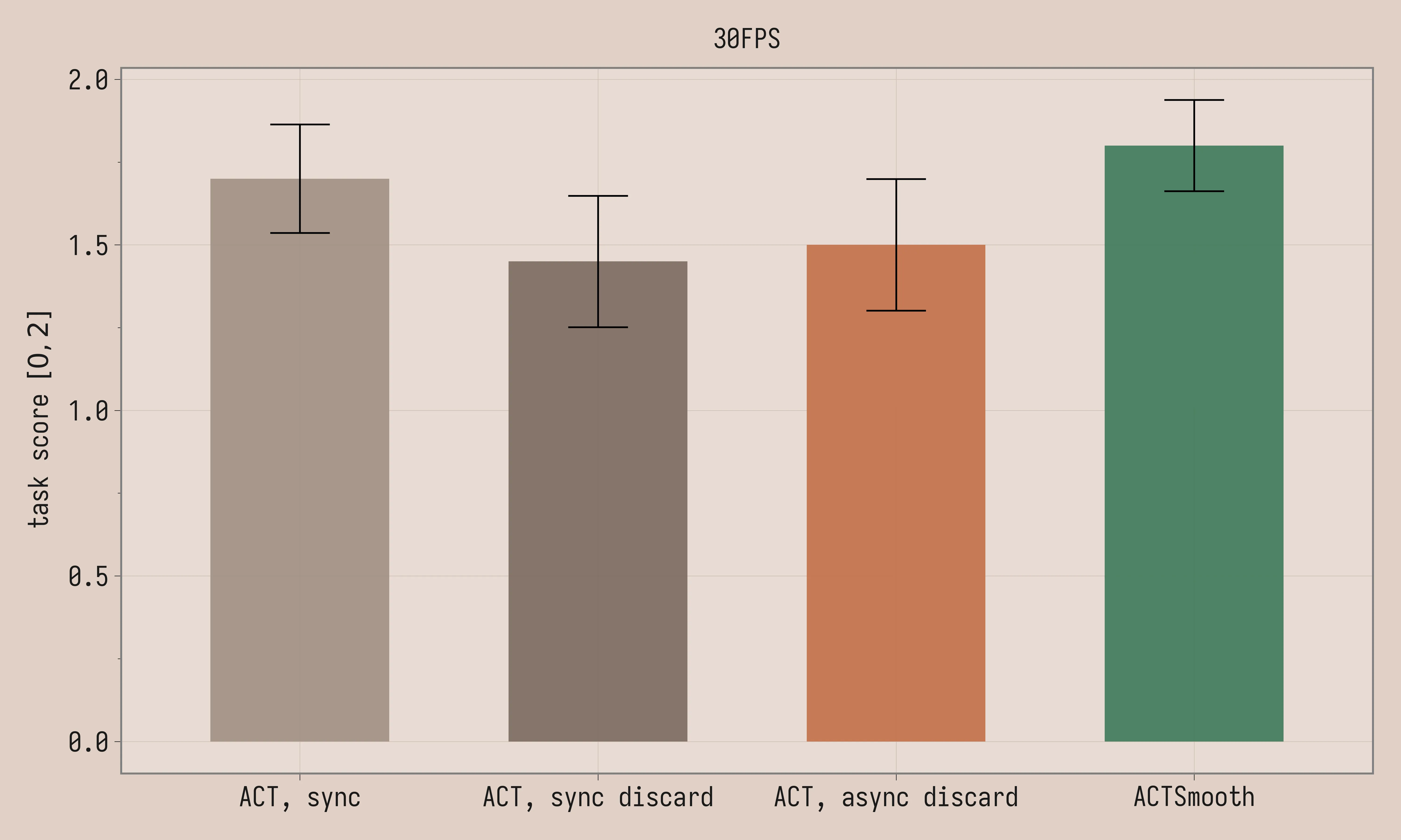
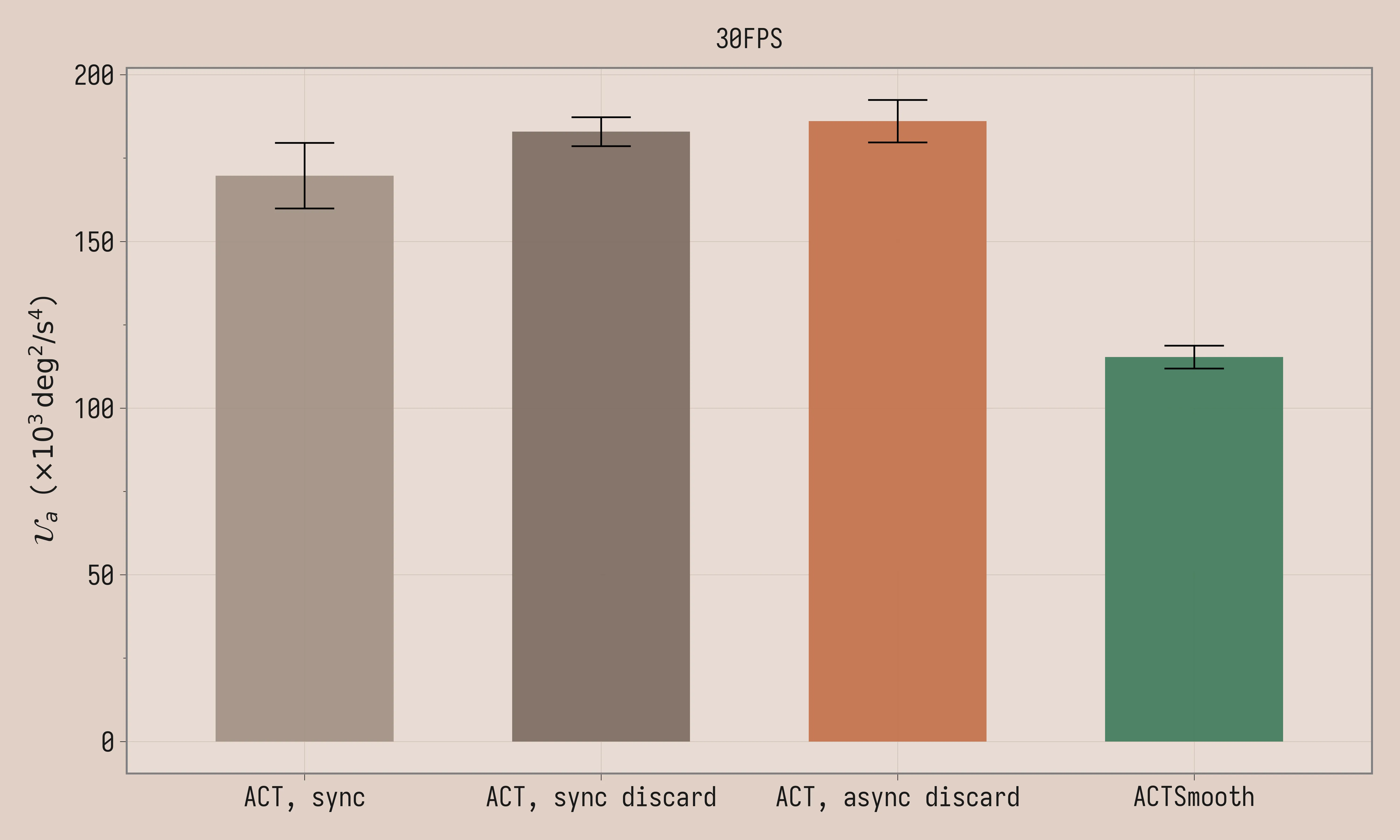
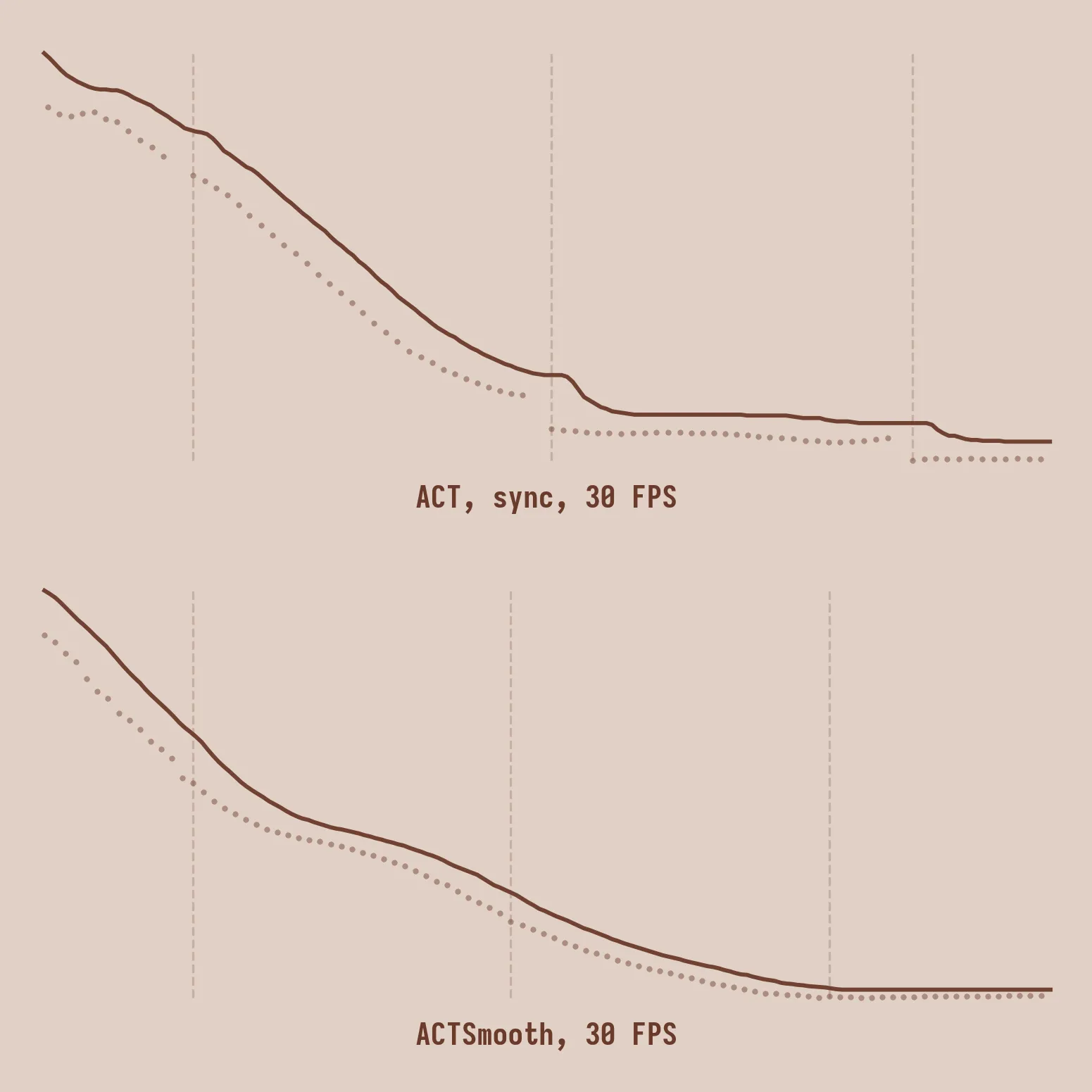
Task scores are comparable between the four methods, given the large standard error. Uniformity of acceleration is meaningfully lower for ACTSmooth. The videos paint a more colorful picture: the policy visibly stalls with synchronous inference, with latency matching, jerk increases because of the larger discontinuities between chunks, while ACTSmooth produces well-behaved trajectories.
Robustness to inference delays
In our setup, inference latency for both vanilla ACT and ACTSmooth is fairly low, around 40ms, but we wanted to see how the ideas scale to potentially larger models or slower hardware. We manually inject inference delays of 100ms and 200ms.
To accommodate larger inference latencies ACTSmooth is retrained with k=4 and D=8 (a separate checkpoint from the D=2 model in the comparison above). The threshold is set to 2, 5, and 8, respectively for 0ms, 100ms, and 200ms of injected delay, for both vanilla ACT with asynchronous latency matching and ACTSmooth (the threshold is lower than D at 0ms and 100ms of injected delay).
Task score:
| Method | 0ms | 100ms | 200ms |
|---|---|---|---|
| ACT, sync, 30FPS | 1.7 ± 0.16 | 1.6 ± 0.18 | 1.9 ± 0.10 |
| ACT, sync discard, 30FPS | 1.4 ± 0.20 | 1.4 ± 0.21 | 1.8 ± 0.14 |
| ACT, async discard, 30FPS | 1.5 ± 0.20 | 1.6 ± 0.18 | 1.5 ± 0.17 |
| ACTSmooth, 30FPS | 1.8 ± 0.12 | 1.6 ± 0.17 | 1.6 ± 0.18 |
\mathcal{U}_a (×10³ deg²/s⁴):
| Method | 0ms | 100ms | 200ms |
|---|---|---|---|
| ACT, sync, 30FPS | 170 ± 9.8 | 159 ± 4.6 | 150 ± 2.6 |
| ACT, sync discard, 30FPS | 183 ± 4.3 | 214 ± 6.6 | 264 ± 11 |
| ACT, async discard, 30FPS | 186 ± 6.4 | 231 ± 6.2 | 260 ± 11 |
| ACTSmooth, 30FPS | 108 ± 4.4 | 112 ± 6.2 | 126 ± 6.9 |
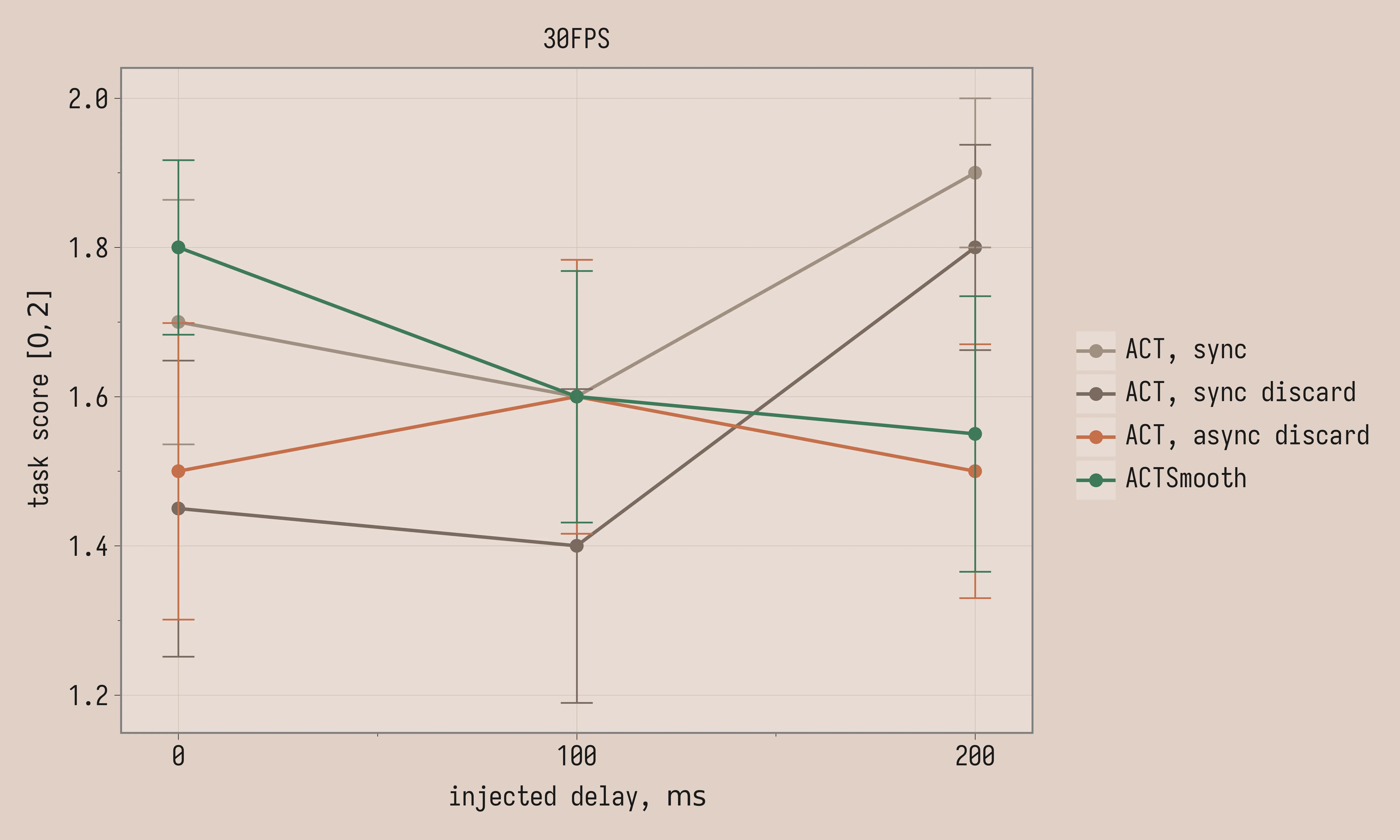
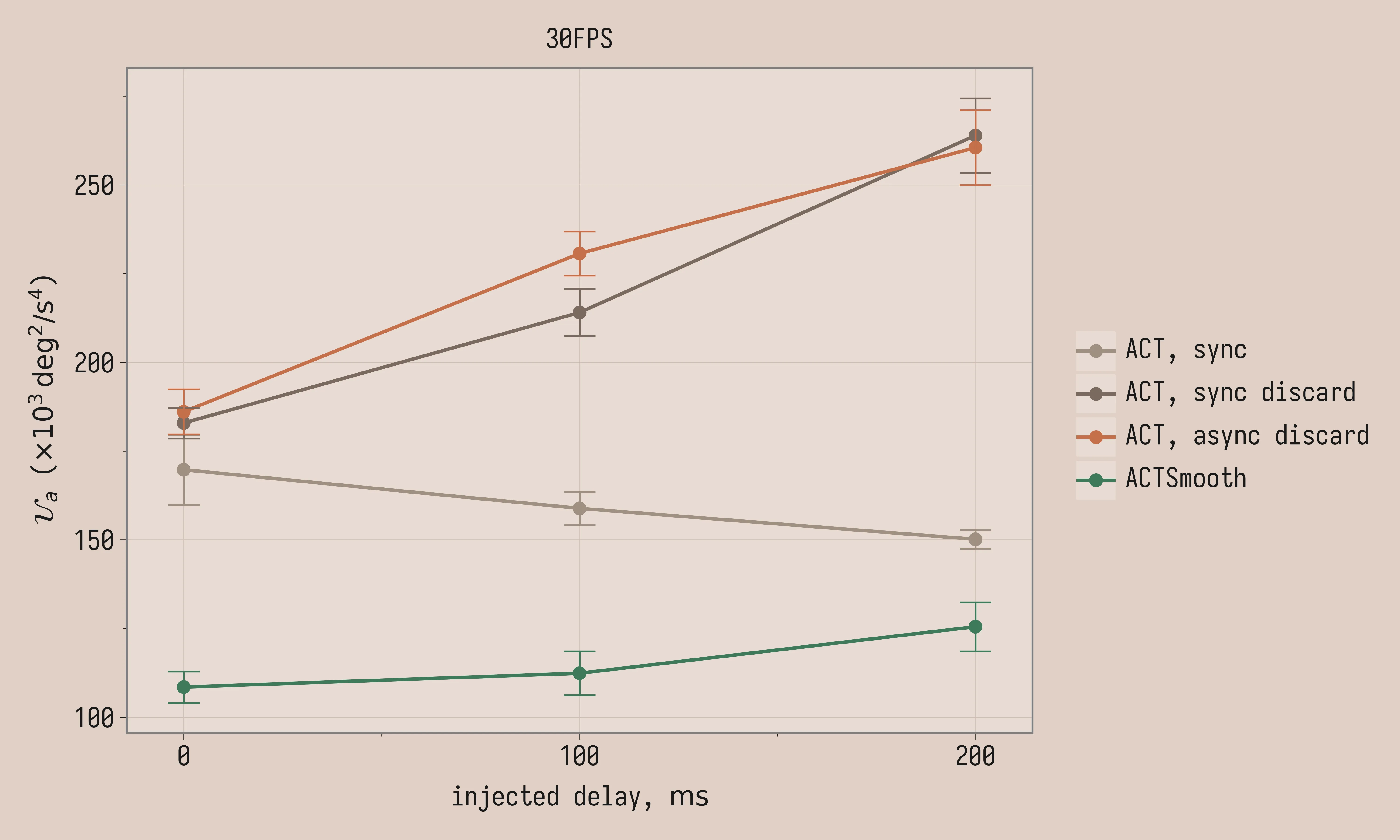
Task score variance is large enough that all conditions are within noise of each other. Instead we see stark differences in the uniformity of acceleration: ACTSmooth is much smoother than other methods and remains smooth at higher latencies, in contrast to vanilla ACT. Uniformity of acceleration improves with added delay for vanilla ACT with synchronous inference; the reason might be that long trajectory stalls contribute lower acceleration variance since the robot does not move. The same does not happen with latency matching, likely because the discontinuities become more severe with longer delays: the robot jumps more aggressively between chunks.
Ablations
We run two ablations for ACTSmooth: removing the relative action representation and removing the past prefix. The baseline is the same policy that we used in Comparison (k = 4 and D = 2), while the other two policies are trained from scratch. The policy without relative actions is trained with k = 4 and D = 2 and absolute joint positions as action representation. The policy without past prefix is trained with k = 0 and D = 2.
| Ablation | Task Score | \mathcal{U}_a (×10³ deg²/s⁴) |
|---|---|---|
| ACTSmooth, 30FPS | 1.8 ± 0.14 | 115 ± 3.4 |
| ACTSmooth, no relative actions, 30FPS | 1.6 ± 0.18 | 168 ± 5.1 |
| ACTSmooth, no past prefix, 30FPS | 1.6 ± 0.18 | 103 ± 6.4 |
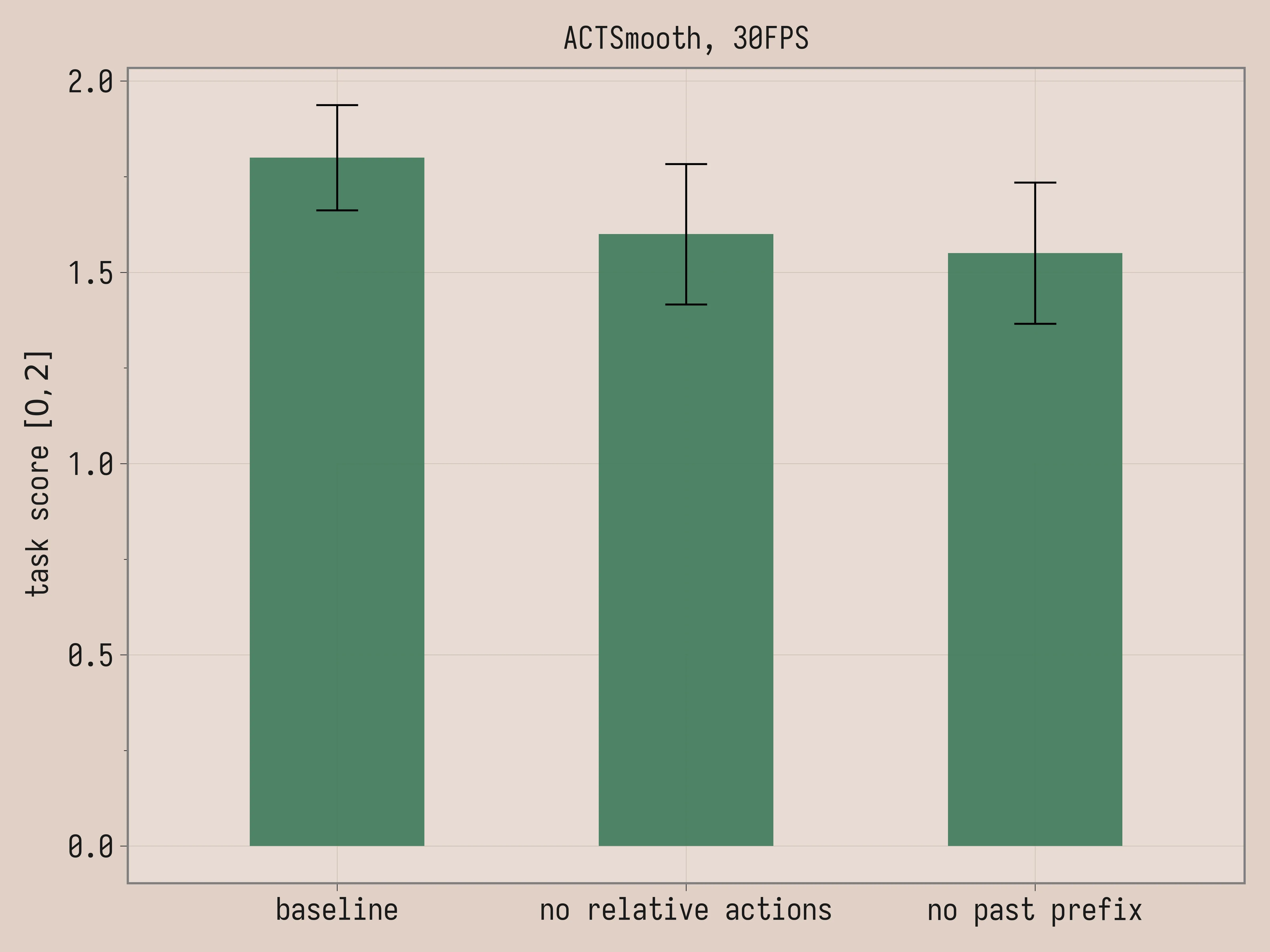
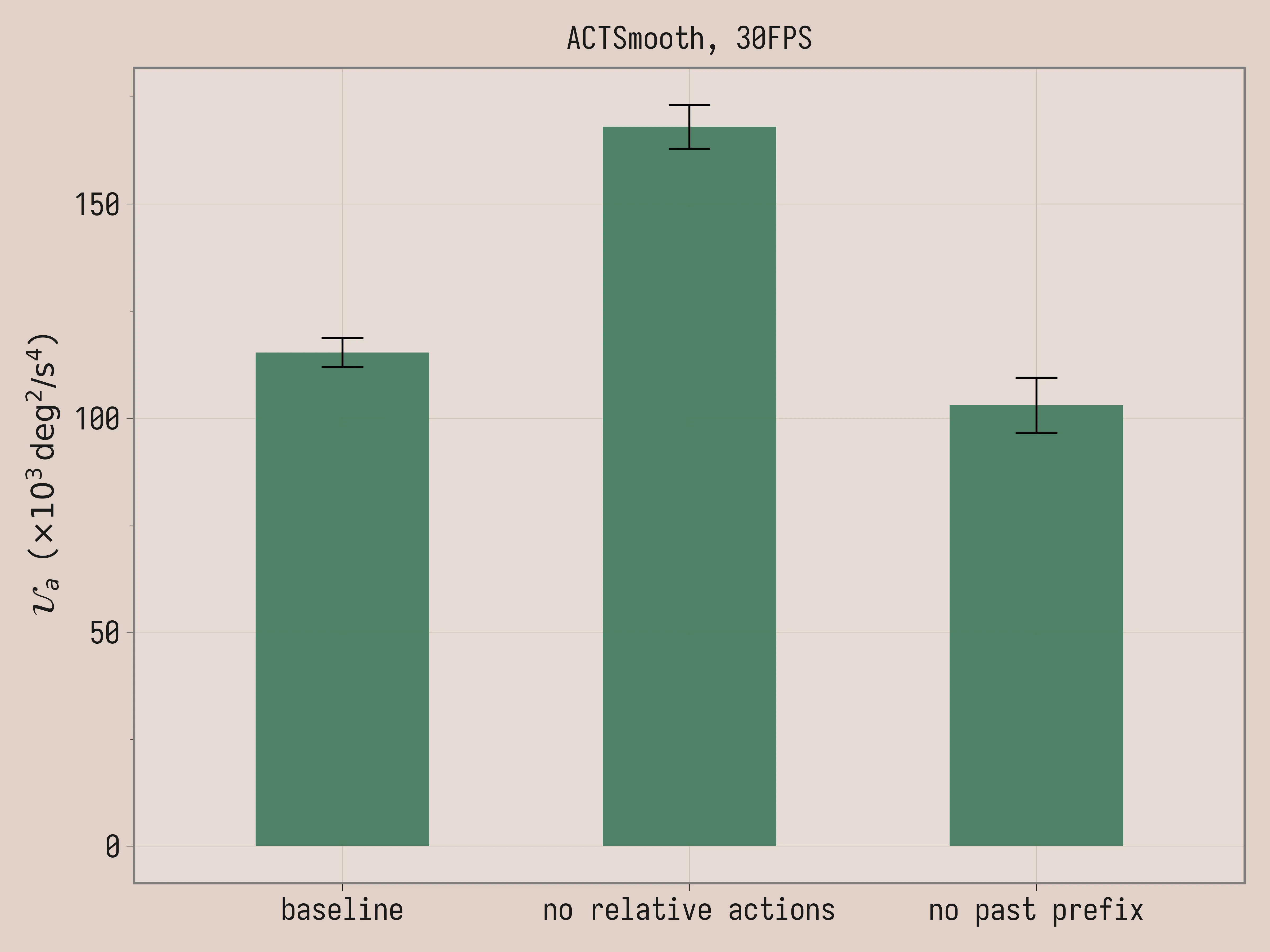
Here the task scores are comparable. The video and the uniformity of acceleration agree that relative actions are essential for the smoothness of ACTSmooth. By contrast, past prefix is a negative result: removing it produces slightly smoother trajectories (103 vs 115 \mathcal{U}_a) with comparable task performance.
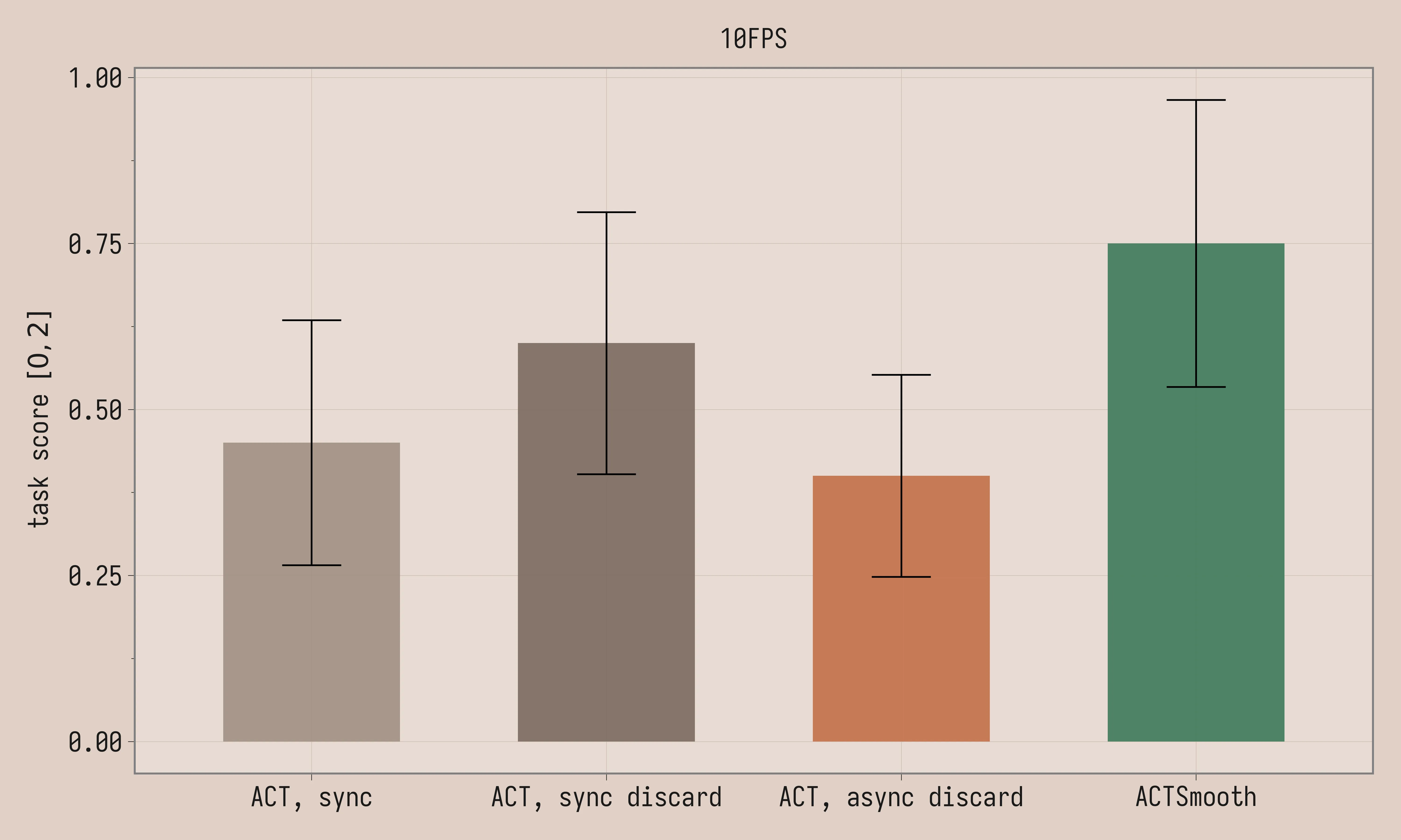
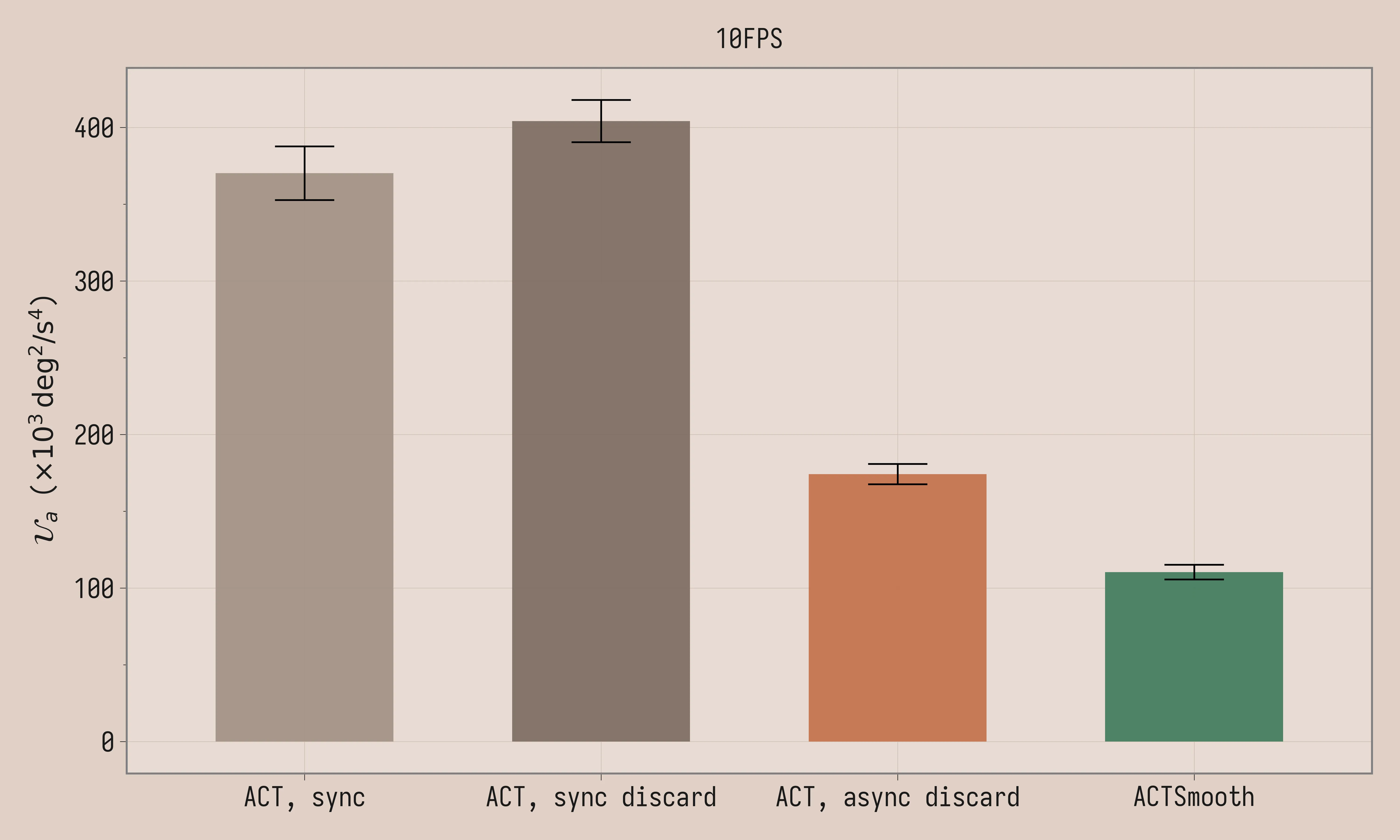
10FPS
We trained the policies on the downsampled 10FPS dataset with chunk length C = 10. ACTSmooth is trained with k=1 and D=2. The threshold is set to 2 for both vanilla ACT with asynchronous latency matching and ACTSmooth (matching D). A key change that enables smooth policies at 10FPS is linear interpolation between commanded actions: commanding a position every 100ms makes the robot stutter through the trajectory. In all asynchronous inference scripts, we linearly interpolate between consecutive actions to effectively command the robot at 30FPS. Given that inference latency in our system is ~40ms and each timestep takes 100ms, we should be fine setting D = 1 in ACTSmooth; instead we set D = 2 so that at chunk switches there is always a future action we can interpolate towards. Note that 30k training steps is likely insufficient for these 10FPS policies; the low task scores suggest that they are undertrained.
| Method | Task Score | \mathcal{U}_a (×10³ deg²/s⁴) |
|---|---|---|
| ACT, sync, 10FPS | 0.4 ± 0.18 | 370 ± 18 |
| ACT, sync discard, 10FPS | 0.6 ± 0.20 | 404 ± 14 |
| ACT, async discard, 10FPS | 0.4 ± 0.15 | 174 ± 6.6 |
| ACTSmooth, 10FPS | 0.8 ± 0.22 | 110 ± 4.8 |
Conclusion
The main motivation of the original RTC paper is to run inference for a 3B-parameter neural network on a powerful remote GPU, where latencies are inevitably in the low hundreds of milliseconds. As we’ve shown, the techniques developed in that paper and further work are useful also for smaller models (30M parameters) running at ~40ms inference latency on the same machine that controls the robot. We were able to visibly improve the robot motion for a simple pick and place task. Directions for future work include evaluating on more varied tasks and directly comparing ACTSmooth to training-time RTC, VLASH, and REMAC applied to equivalent base models.
This was a helpful exercise and I learned a ton. Robot learning is fun because you often have to work across different systems to achieve better results; in this case, the solution for smooth policies was not isolated to the model or to the inference script but required thinking and iterating across both of them.
You can find the project on GitHub at: https://github.com/giacomoran/lerobot-policy-act-smooth. It follows the Bring Your Own Policies instructions from LeRobot, so you can easily train ACTSmooth on your own tasks.
I’d love to connect to more people building robots in Europe/Italy/Veneto. The best way to get updates on my work is x dot com.
References
- Zhao, 2023 - (ALOHA, ACT) Learning Fine-Grained Bimanual Manipulation with Low-Cost Hardware
- Black, 2025 - (RTC) Real-Time Execution of Action Chunking Flow Policies
- Black, 2025 - (Training-Time RTC) Training-Time Action Conditioning for Efficient Real-Time Chunking
- Tang, 2025 - VLASH: Real-Time VLAs via Future-State-Aware Asynchronous Inference
- Wang, 2026 - (REMAC) Real-Time Robot Execution with Masked Action Chunking
- Liu, 2026 - (TERM) Trustworthy Evaluation of Robotic Manipulation A New Benchmark and AutoEval Methods
- Chi, 2024 - (UMI) Universal Manipulation Interface In-The-Wild Robot Teaching Without In-The-Wild Robots